Introduction

In this post, we breifly summarize the basic concepts related to graph algorithm. Then, we study topological sort to make the graph concepts into practice.

Graph Basics

Definitions

• A graph \(G = (V,E)\) consists of a set of vertices \(V\), and a set of edges \(E\).
• Each edge (i.e., arcs) is a pair \((v,w)\), where \(v,w \in V\).
• Given an edge \(e = (u,v)\), the vertex \(u\) is its source, and \(v\) is its sink.
• If the pair is ordered, then the graph is directed (i.e., digraphs).
• Vertex \(w\) is adjacent to \(v\) iff \((v,w) \in E\).

• A path in a graph is a sequence of vertices \(w_1, w_2, w_3, \dots, w_N\) such that \((w_i, w_{i+1}) \in E\) for \(1 \le i < N\). The length of such path is the number of edges on the path, which is equal to \(N - 1\).

• A simple path is a path such that all vertices are distinct, except that the first and last could be the same.
• If there is a path from \(u\) to \(v\), \(v\) is said to be reachable from \(u\).
• A cycle in a graph:
  • For directed graph, a cycle is a path of length at least 1 such that vertices \(w_1 = w_N\).
  • For undirected graph, we require edges to be distinct
    • reasoning: the path \(u,v,u\) in an undirected graph should not be considered a cycle because \((u,v)\) and \((v,u)\) are the same edge.
• A directed acyclic graph (DAG) is a directed graph in which there are no cycles (i.e., paths which contain one or more edges and which begin and end at the same vertex)
  • Vertices in a DAG which have no incoming edges are referred to as sources
  • Vertices which have no outgoing edges are referred to as sinks
• connected:
  • An undirected graph is connected if there is a path from every vertex to every other vertex.
  • A directed graph is connected if it contains a directed path from \(u\) to \(v\) or a directed path from \(v\) to \(u\) for every pair of vertices \(u\) and \(v\).
• A directed graph is strongly connected if it contains a directed path from \(u\) to \(v\) and a directed path from \(v\) to \(u\) for every pair of vertices \(u\) and \(v\).
• If a directed graph is not strongly connected, but the underlying graph (without direction to the arcs) is connected, then the graph is said to be weakly connected.
• For a graph \(G\), a connected component is a maximal set of vertices \(C\) such that each pair of vertices in \(C\) is connected in \(G\). Every vertex belongs to exactly one connected component.
• A complete graph is a graph in which there is an edge between every pair of vertices.

• Indegree of a vertex \(v\) is the number of edges \((u,v)\)
• Outdegree of a vertex \(v\) is the number of edges \((v,u)\)

Representation

• Adjacency matrix: use a \(|V| \times |V|\) matrix indexed by vertices, with a 1 indicating the presence of an edge (i.e. For each edge \((u, v)\), we set A[u][v] to true; otherwise the entry in the array is false). If the edge has a weight associated with it, then we can set A[u][v] equal to the weight and use either a very large or a very small weight as a sentinel to indicate nonexistent edges.

  • Disadvantage: we require graph to be dense: \(|E| = \Theta(|V|^2)\), which is very unlikely.

• Adjacency list: For each vertex, we keep a list of all adjacent vertices. For undirected graph, each edge \((u,v)\) appears in two lists

  • Advantage: only requires \(O(|E|+|V|)\) space.

• Edge Lists: we represent the graph as an array of \(|E|\) edges. For example, for an undirected edge connects \(0\) and \(1\), we can represent it as [0,1].

Topological Sort

Definition and Properties

• We have following two equivalent definitions:
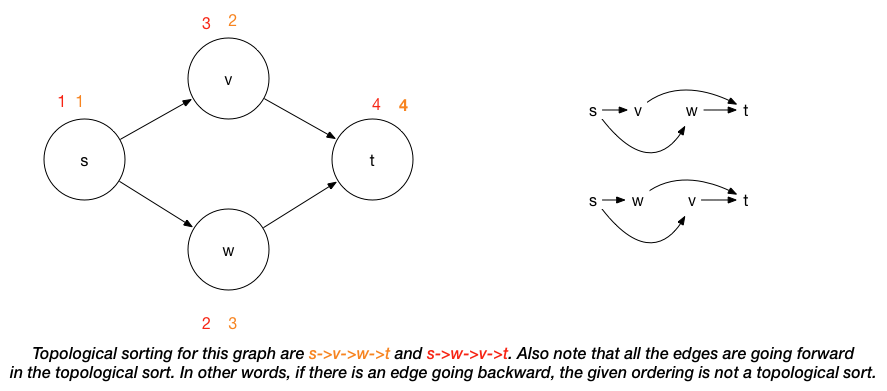
  • Def 1: A topological sort is an ordering of vertices in a DAG such that if there is a path from \(v_i\) to \(v_j\), then \(v_j\) appears after \(v_i\) in the ordering.
  • Def 2: A topological ordering of a DAG \(G\) is a labeling \(f\) of \(G\)'s nodes such that:
    • The \(f(v)\)'s are the set \({1,2, \dots, n}\)
    • \((u,v) \in G \implies f(u) < f(v)\)

• Application: sequence tasks while respecting all precedence constraints. (e.g. course prerequisite structure can be represented as a graph. A topological ordering of these courses is any course sequence that does not violate the prerequisite requirement.)

• If G has a cycle, there is no topological sort: since for two vertices \(v\) and \(w\) on the cycle, \(v\) precedes \(w\) and \(w\) precedes \(v\). On ther other hand, if there is no directed cycle in the graph, we can compute topological sort in linear time (\(O(|V|+|E|)\)).

• Topological sorting is not necessary unique as shown in the picture above.

DFS Approach

The basic idea of computing the topological ordering is following:

• Let \(v\) be a sink vertex of \(G\)
• set \(f(v) = n\)
• recurse on \(G - {v}\)

There are some proofs we need to show for the correctness of the procedure:

• Every directed acyclic graph has a sink vertex

  Suppose the DAG doesn't have a sink vertex, that means every single vertex has at least one outgoing arc. We can start with arbitrary vertex and follow its outgoing arc to the next vertex. Since there is no sink vertex in our graph, we can repeatedly follow the outgoing arc of the vertex. Suppose there are \(N\) nodes in the graph and by following edges for \(N\) times, we reach the \(N+1\)th vertex. Since among the \(N+1\) nodes, there are only \(N\) distinct nodes. By the pigeonhole principle, we must have visted some vertex twice. By following the nodes and visited some node twice, we show that the graph contains a directed cycle, which is a contradiction.

• During each recursion step, we can find a sink vertex

  For a DAG, if we delete one or some of the vertices, we still have DAG (i.e., we cannot create a directed cycle). Thus, in each recursion step, we always have DAG. Then, by the previous observation, during each recursion step, we can find a sink vertex.

• The above steps do produce topological ordering

  By topological ordering, we know that all the edges have to go forward. Intutively, we always want to assign the sink vertex of the graph to the final position because otherwise there is going to be an outgoing arc of the node and the node that the outgoing arc points to will be assigned a lower position, which violates the topological ordering (i.e. edge goes backward). In our procedure, when a node \(v\) is assigned to position \(i\), that means we only have \(i\) nodes remaining and \(v\) is the sink vertex. This implies that all of outgoing arcs and the corresponding nodes are deleted and assigned higher positions. So for every vertex, by the time it actually gets assigned a position, it's a sink and it only has incoming arcs from the as yet unsigned vertices. It's outgoing arcs all go forward to vertices that were already assigned higher positions, and got deleted previously from the graph.

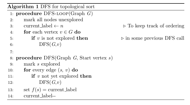
To implement the procedure above, we use the DFS:

There are several points we need to note here:

• We set \(f(s) = \text{current_label}\) right before we about to pop the call stack. At that point, for every edge \((s,v)\), there is no such \(v\) that we haven't explored. That means there are no outgoing edges, which indicate that \(s\) is a sink and thus we can assign it a labeling.

• Running time: \(O(|E|+|V|)\) (we only visit each vertex in the graph once and we look at each edge once as well)

• Correctness: we want to show that this DFS algorithm can correctly produce topological ordering. Topological ordering requires that for an edge \((s,v)\), \(f(s) < f(v)\). There are two possible cases for DFS: 1) \(s\) get visited first 2) \(v\) get visited first. For the first case, since there is an edge from \(s\) to \(v\), DFS will recursively call on \(v\). In other words, DFS call on \(v\) will finish before the DFS call on \(s\). Thus, \(v\) will get a label larger than \(s\) and the topological ordering is satisfied. For the second case, since there is no cycle in DAG, \(s\) will not get discovered. Thus, \(s\) will be visited later than \(v\). By the same reasoning as the first case, we still have the topological ordering.

BFS Approach

Not surprisingly, we can find topological ordering of a graph using BFS as well. Instead of finding the sink vertex each time (i.e. the vertex with outdegree = 0), we find the source vertex (i.e. the vertex with indegree = 0) each time in BFS. The basic steps to compute the topological ordering follows:

• Let \(s\) be a source vertex of \(G\)
• set \(f(s) = 1\)
• recurse on \(G - {s}\)

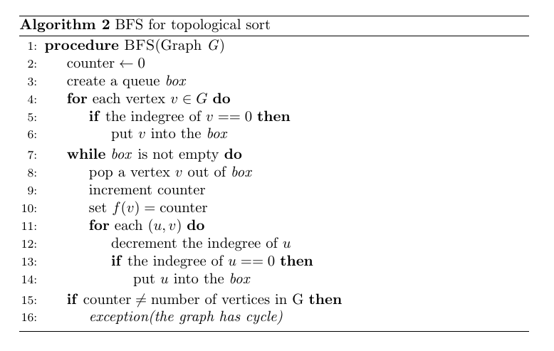
We omit the proofs of the properties in BFS as the proofs will mirror with the ones for DFS. We can use the BFS to implement the procedure above:

There are several points we need to note here:

• In the basic version, we pick a source vertex of \(G\) each time and assign the label. Inevitably, we will compute all the indegree of all nodes in the graph to find the source vertices. However, not all nodes' indegrees will be updated. To save this duplicate calculation, we use a queue (box).

• Running time: \(O(|E|+|V|)\) (We visit each edge once and for each node, we visit twice: compute the inital indegree; assign the labeling)

• Correctness: this BFS will prodcue the topological ordering because for an edge \((s,v)\), we will always visit \(s\) before visiting \(v\). Without removing \(s\) first, \(v\) will always have an incoming edge, which will not make \(v\) a source vertex. Since we assign the labeling in the increasing order, \(f(s) < f(v)\). Thus, we produce a topological ordering.

As one can see the difference between DFS and BFS is that: for DFS, we start with the sink vertex and assign the label of the vertices in the decreasing order (i.e. start from \(n\) and until \(1\)). However, for BFS, we start with the source vertex and assign the label of the vertices in the increasing fashion (i.e. start from \(1\) and until \(n\)).

Reference

• "Data Structures and Algorithm Analysis in C++, 4th Edition" by Mark A. Weiss (we use MAW (cpp) for short in the future)
• "Elements of Programming Interviews: The Insiders' Guide" by Adnan Aziz, Tsung-Hsien Lee, and Amit Prakash, p.342 - 346 (we use ATA for short in the future)
• Topological Sort on Coursera