Motivation

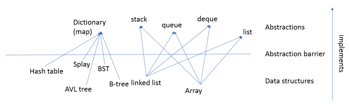
In the previous chapter, we implement the dictionary (map) ADT using tree structure. A typical find or insert operations require \(O(\log N)\) time. However, this is not good enough compared with \(O(1)\) time. This is place where hash tables implementation can shine. Hash tables is a data structure that is designed for \(O(1)\) find, insert, and delete operations. The only downside compared hash tables with tree structure is the ill support for ordering elements.

General Idea

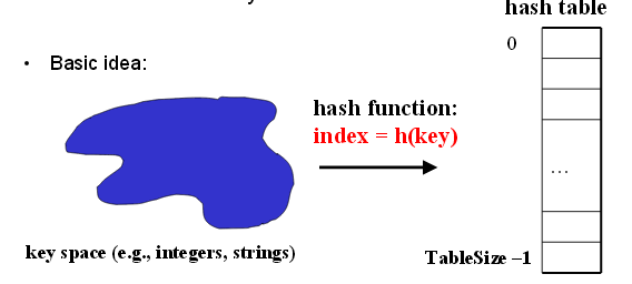
A hash table is an array of some fixed size. Then we use hash function to map each key (i.e. a key is a string with an associated value) into some number in the range 0 to Tablesize-1 and place it in the appropriate cell.

Ideally, two distinct keys get different cells. However, this is not possible because there are a finite number of cells and a virtually infinite supply of keys. Thus the key concern for hash table data structure is how to distribute the keys evenly among the cells. This issue is addressed from two ways: 1) pick a good hash function to avoid collision (i.e. two keys hash to the same value) 2) use a good strategy to redistribute keys when collision happens.

Hash function

Hash function is a mapping from the element key (string or number) to an integer (the hash value). The output of the hash function must always be less than the size of array and should be as evenly distributed as possible. One thing to note here is that the pick of hash function has high dependency on the actual content of the key set.

We list some key points from the chapter here:

• Choose the table size of the hash table to be the prime.

The rationale for this is that real-life data tends to have pattern, and "multiples of 61" are probably less likely than "multiples of 60". In addition, quadratic hashing is an efficient collision strategy to use (compared with linear hashing, double hashing) and it requires the table size to be the prime.

• When we deal with string keys, we may use \(\big(\sum_{i=0}^{k-1} s_i \cdot 256^i \big) \bmod TableSize\) as our function.

Here we use 256 because char data is 1 byte. Other hash function may be adding up the ASCII values ofthe characters in the string. However, this doesn't work well because if string keys are short, it will not hash evenly to all of the hash table (see MAW p.151) and different character combinations hash to same value (i.e. "abc", "bca" all add up to the same value).

The slides listed in the reference section offer some examples on hash function pick if we know the keys beforehand (i.e. if keys \(s\) are the real numbers uniformly distributed over \(0 \leq s < 1\)).

Collision strategy

A collision occurs when two different keys hash to the same value. By the nature of dictionary ADT, we cannot store both data records in the same cell in the array. So, we need to come up a strategy to resolve collision and try our best to make the keys evenly distribute among the table. There are two main strategies discussed in the chapter: separate chaining and open addressing.

Separate chaining

Note

Sometimes separate chaining is also referred as "open hashing", which means that none of the objects are stored inside the hash table's internal array. For example, objects are stored in lists of buckets for hash table implementng the separate chaining.

Separate chaining is to keep a list (chain or bucket) of all elements that hash to the same value. In other words, each hash table cell holds pointer to linked list of records with same hash value. When collision happens, we insert the hash value of the key to the corresponding linked list of the cell that hash value should be stored. When we want to find an item, we compute the hash value, then do find on linked list.

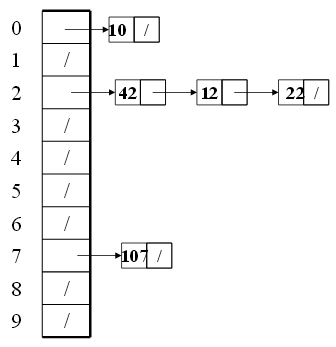
Here the worst case time happens for find operation, which can take linear time. However, this can happen in the extreme rare case (bad luck or bad hash function). Of course, we can build a balance tree instead of a linked list on each cell to shrink the find time. But, the structure overhead and the compelxity of insert may make this effort not worth it.

The average length of chained list = \(\lambda\). Thus, the average time for accessing an item = \(O(1) + O(\lambda)\). So, we want \(\lambda\) to be smaller than 1 but close to 1 if good hashing function. Thus, the general rule for separate chaining hashing is to make the table size about as large as the number of elements expected (let \(\lambda \approx 1\)).

Note

Actually, separate chaining doesn't restrict us to use the list to chain the objects together. We can use a tree to organize the elements that have the same hash value.