B-Tree
This is the summary of B tree part in MAW Chapter 4.
Motivation
So far we have assumed that an entire data structure can be stored in the main memory. However, this is not true in reality because if we have more data than can fit in main memory, we have to store data structure on disk. In this case, number of disk accesses will dominate the running time because they are very expensive comparing with the processor speed. Then, when we design a data structure, we have to try our best to minimize the number of disk accesses. Under the context of tree structure, B-tree is a structure that tries to read as much information as possible in every disk access operation.
Concept
B-tree is by far the most chaoatic defined structure in the sense that different people have slightly different definitions. I’ll follow MAW’s definition and points out how MAW’s definition is different from the other commonly seen definition.
A B-tree of order \(M\) is a tree with the following structural properties:
- The leaves contain all the actual data, which are either the key temselves or pointers to records containing the keys.
- The root is either a leaf (when tree has \(\le L\) items) or has between \(2\) and \(M\) children.
- All nonleaf nodes (except the root) have between \(\lceil{M/2}\rceil\) and \(M\) children (at least half full).
- All leaves are the same depth and have between \(\lceil{L/2}\rceil\) and \(L\) sorted data items, for some L (at least half full).
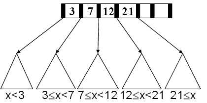
- The nonleaf nodes have room for up to \(M-1\) keys to guide the searching; key \(i\) represents the smallest key in subtree \(i+1\).
In MAW, the definition of B-tree is essentially known as \(B^+-\)tree. Technically, the real B-tree has the key property that the actual data to be stored in both leaves and internal nodes, which is not the case in our definition. In some \(B^+-\)tree definition, the leaves are connected as a linked list so that we don’t have to restart the search from the root once we already traverse down to the leaf if we want a record that is on a leaf really close to the leaf we currently at.
Examples
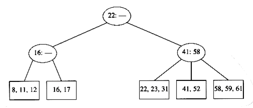
Some typical examples in B-tree are of order 4 (known as 2-3-4 tree) and 3 (known as 2-3 tree).
B-tree is a structure that is widely used in the database system. The following picture shows a more real B-tree example. Suppose we have a large customer table with gigabytes of data and an index is created on the phone number column of the customer table to speed up search. Phone numbers stored in sorted order with information (page and slot) on where the rest of the customer information can be found in the customer table.
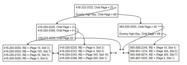
In this example, once we continue down the tree and locate the phone number we are searching for, we use the RID to fetch the rest of the customer record from the table. In this case, we use 4 page accesses to get the full customer record from the table.
Operations
- Find:
For find, we basically do binary search on each node to decide what subtree we should go to search.
- Insertion:
The major unique manipulation is we may need to split the node at the leaves and recursives make the new parent nodes (by pushing a key up to its parent) to the root. Other strategies regarding nodes overloaded also exist but this one is classic textbook.
- Deletion:
I have to say deletion is the most messy one and people may always want to talk about it conceptually instead of getting hands dirty to actually implement one. Stanford paper listed in the reference section do a concrete implementation but the route they use is to implement a real-life B-tree deletion which may be complicated for the learner.
The strategy we use for deletion is that we want to find the key to be deleted and remove it first. Then, if the leaf underflows, we borrow from a neighbor. If leaf underflows and can’t borrow, we merge nodes and delete parent.
Runtime analysis
We first show that height \(H\) is logarithmic in number of data items \(N\). Let \(M \ge 2\). Because all nodes are at least half full (except root may have only 2 children) and all leaves are at the same level, the minimum number of data items \(N\) for a height \(H\) tree is
Then for a B-tree of order \(M\)
- Each internal node has up to \(M-1\) keys to search
- Each internal node has between \(\lceil{M/2}\rceil\) and \(M\) children
- Depth of B-tree storing \(N\) items is \(O(\log_{\lceil{M/2}\rceil}N)\)
Find then takes \(O(\log M)\) to do binary search on each node to determine which branch to take. Then the total time is \(O(depth \times \log M)\) = \(O(\log N)\) because \(M\) is small compared to \(N\).
Insertion and deletion doesn’t different from \(O(\log N)\) because the unique manipulation takes constant amount of work and the number of times this unique manipulation is proportional to the height of tree.
Pros & Cons of data structure
What makes B-trees so disk friendly?
-
Many keys stored in one node
- All brought into memory in one disk access
- Pick \(M\) wisely. See MAW’s Java version (3rd edition) p.149 for an example.
- Makes the binary searhc over \(M-1\) keys totally worth it.
-
Internal nodes contain only keys
- All find wants only one data item. So only bring one leaf of data items into memory.
- Data-item size doesn’t affect what \(M\) is. We determine \(M\) only by how many keys can be packed into a disk block (node). Thus, the key size, the children pointer size, and the block size are the only factors here.
Links to resources
Here are some of the resources I found helpful while preparing this article:
- MAW Chapter 4
- Lecture slides 15, 8, and 9 from U.Washington
- Yale pinewiki on B-tree
- Stanford B-tree implementation paper